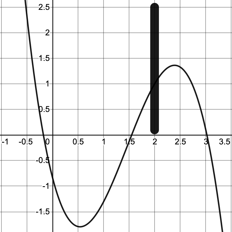
In Figure 1 the graph of a function is given, but something is wrong. The graphic card failed and one portion did not render properly. We can’t see what is happening in the neighborhood of \(x=2\text{.}\)
Figure1.A graph of a function that has not been rendered properly.
(a)
Imagine moving along the graph toward the missing portion from the left, so that you are climbing up and to the right toward the obscured area of the graph. What \(y\)-value are you approaching?
0.5
1
1.5
2
2.5
(b)
Think of the same process, but this time from the right. You’re falling down and to the left this time as you come close to the missing portion. What \(y\)-value are you approaching?
0.5
1
1.5
2
2.5
Activity1.1.2.
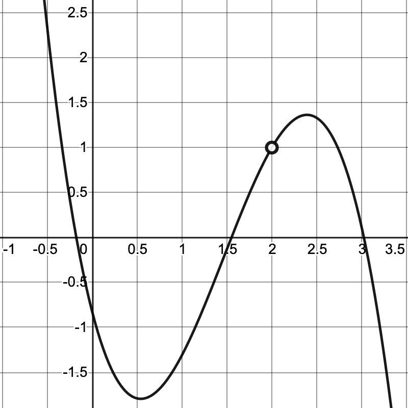
In Figure 2 the graphic card is working again and we can see more clearly what is happening in the neighborhood of \(x=2\text{.}\)
Figure2.A graph of a function that has rendered properly
(a)
What is the value of \(f(2)\text{?}\)
(b)
What is the \(y\)-value that is approached as we move toward \(x = 2\) from the left?
0.5
1
1.5
2
2.5
(c)
What is the \(y\)-value that is approached as we move toward \(x = 2\) from the right?
0.5
1
1.5
2
2.5
Remark1.1.3.
When studying functions in algebra, we often focused on the value of a function given a specific \(x\)-value. For instance, finding \(f(2)\) for some function \(f(x)\text{.}\) In calculus, and here in Activity 1.1.1 and Activity 1.1.2, we have instead been exploring what is happening as we approach a certain value on a graph. This concept in mathematics is known as finding a limit.
Activity1.1.4.
Based on Activity 1.1.1 and Activity 1.1.2, write your first draft of the definition of a limit. What is important to include? (You can use concepts of limits from your daily life to motivate or define what a limit is.)
Definition1.1.5.
Given a function \(f\text{,}\) a fixed input \(x = a\text{,}\) and a real number \(L\text{,}\) we say that \(f\) has limit \(L\) as \(x\) approaches \(a\), and write
\begin{equation*}
\lim_{x \to a} f(x) = L
\end{equation*}
provided that we can make \(f(x)\) as close to \(L\) as we like by taking \(x\) sufficiently close (but not equal) to \(a\text{.}\) If we cannot make \(f(x)\) as close to a single value as we would like as \(x\) approaches \(a\text{,}\) then we say that \(f\) does not have a limit as \(x\) approaches \(a\text{.}\)
Activity1.1.6.
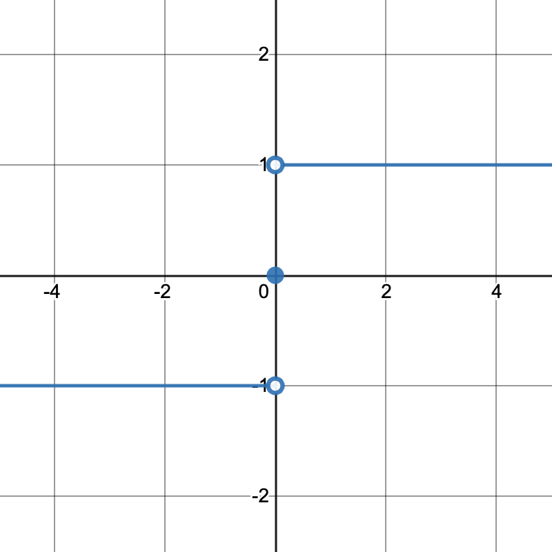
Figure3.A piecewise-defined function
What is the limit as \(x\) approaches \(0\) in Figure 3?
The limit is 1
The limit is -1
The limit is 0
The limit is not defined
Definition1.1.7.
We say that \(f\) has limit \(L_1\) as \(x\) approaches \(a\) from the left and write
provided that we can make the value of \(f(x)\) as close to \(L_1\) as we like by taking \(x\) sufficiently close to \(a\) while always having \(x \lt a\text{.}\) We call \(L_1\) the left-hand limit of \(f\) as \(x\) approaches \(a\text{.}\) Similarly, we say \(L_2\) is the right-hand limit of \(f\) as \(x\) approaches \(a\) and write
provided that we can make the value of \(f(x)\) as close to \(L_2\) as we like by taking \(x\) sufficiently close to \(a\) while always having \(x \gt a\text{.}\)
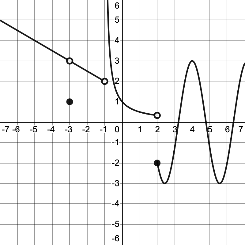
For which \(x\)-values does the overall limit exist? Select all. If the limit exists, find it. If it does not, explain why.
\(\displaystyle -3\)
\(\displaystyle -1\)
\(\displaystyle 2\)
\(\displaystyle 4\)
Activity1.1.10.
Sketch the graph of a function \(f(x)\) that meets all of the following criteria. Be sure to scale your axes and label any important features of your graph.
\(\displaystyle \lim_{x\to 5^-} f(x)\) is finite, but \(\displaystyle \lim_{x\to 5^+} f(x)\) is infinite.
\(\displaystyle \lim_{x\to -3} f(x)=-4\text{,}\) but \(f(-3)=0\text{.}\)
\(\displaystyle \lim_{x\to -1^-} f(x)=-1\) but \(\displaystyle \lim_{x\to -1^+} f(x)\neq-1\text{.}\)
Theorem1.1.11.
Suppose that:
for an interval around \(x=a\text{,}\) we have that \(f(x) \leq g(x) \leq h(x) \) ;
the limit as \(x\) approaches \(a\) of \(f(x) \) is equal to the same value \(L\) as the limit of \(h(x)\text{,}\) so \(\displaystyle\lim_{x\to a} f(x) = L =\lim_{x\to a} h(x) .\)
Then, the limit of \(g(x)\) as \(x \to a\) is also \(L\text{,}\) so \(\displaystyle\lim_{x\to a} g(x) = L \text{.}\)
Activity1.1.12.
In this activity we will explore a mathematical theorem, the Squeeze Theorem Theorem 1.1.11.
(a)
The part of the theorem that starts with “Suppose…” forms the assumptions of the theorem, while the part of the theorem that starts with “Then…” is the conclusion of the theorem. What are the assumptions of the Squeeze Theorem? What is the conclusion?
(b)
The assumptions of the Squeeze Theorem can be restated informally as “the function \(g\) is squeezed between the functions \(f\) and \(h\) around \(a\text{.}\)” Explain in your own words how the two assumptions result into a “squeezing effect.”
(c)
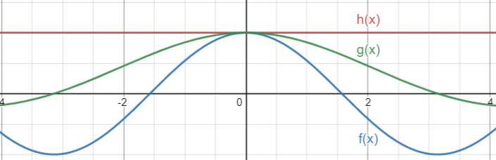
Let’s see an example of the application of this theorem. First examine the following picture. Explain why, from the picture, it seems that both assumptions of the theorem hold.
Figure5.A pictorial example of the Squeeze Theorem.
(d)
Match the functions \(f(x), g(x), h(x)\) in the picture to the functions \(\cos(x), 1, \frac{\sin(x)}{x}\text{.}\)
(e)
Using trigonometry, one can show algebraically that \(\cos(x) \leq \frac{\sin(x)}{x} \leq 1 \) for \(x\) values close to zero. Moreover, \(\displaystyle\lim_{x \to 0} \cos(x) = \cos(0)=1\) (we say that cosine is a continuous function). Use these facts and the Squeeze Theorem, to find the limit \(\displaystyle\lim_{x\to 0} \frac{\sin(x)}{x} \text{.}\)